
Excel is a shockingly tough tool – if you know the way to leverage it. With such a lot of purposes and components choices, there’s one thing new to be informed each day.
The INDEX/MATCH components allow you to to find information issues temporarily with no need to manually seek for them and chance making errors.
![Download 10 Excel Templates for Marketers [Free Kit]](https://wpfixall.com/wp-content/uploads/2021/07/9ff7a4fe-5293-496c-acca-566bc6e73f42.png.webp)
Let’s dive into how that components works and evaluation some useful use circumstances.
Figuring out INDEX and MATCH Purposes Personally
Prior to you’ll be able to know the way to make use of the INDEX and fit components, it’s precious to know the way every serve as works by itself. That may be offering some readability on how each paintings in combination as soon as mixed.
The INDEX serve as returns a price or the connection with a price inside a desk or vary in line with the rows and columns you specify. Bring to mind this serve as as a GPS – it is helping you to find information inside a record however first, you wish to have to slender down the hunt space the usage of rows and columns.
The MATCH serve as identifies a selected merchandise in a variety of cells then returns the relative place of that merchandise within the vary or the precise fit.
As an example, say the variability A1:A4 accommodates the values 15, 28, 49, 90. You need to know the way the quantity “49” is relative to all values inside the vary. You might write the components =MATCH(49,A1:A4,0) and it might go back the quantity 3 as it’s the 3rd quantity within the vary. The 0 within the components represents “precise fit.”
Now that we’ve were given the fundamentals out of the way in which, let’s get into mix the components and use it for more than one standards.
Methods to Use the INDEX and MATCH System with A couple of Standards
The components for the INDEX/MATCH components is as follows: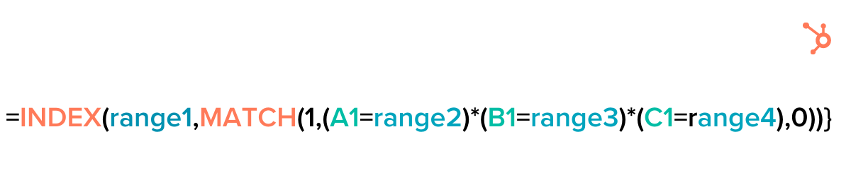
Right here’s how every serve as works in combination: Fit reveals a price and will provide you with its location. It then feeds that data to the INDEX serve as, which turns that data right into a consequence.
To look it in motion, let’s use an instance.
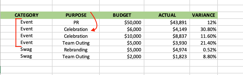
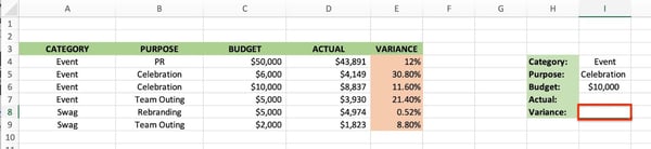
This Excel sheet includes a advertising price range for 2 classes: Occasions and corporate swag items. There are 4 functions: Public members of the family (PR), birthday party, staff time out, and rebranding. The sheet additionally contains the outlined price range and the real expense for every class.
That is the place the INDEX and MATCH components is useful when the usage of it for more than one standards. You’ll be able to temporarily uncover the answer(s) you’re on the lookout for and prohibit errors that may occur when looking manually.
Say you need to understand the variance for an match that had a goal of birthday party with the cheap of 10,000 – right here’s the way you’d do it.
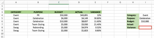
First, keep in mind of the row numbers and columns. The solution you’re on the lookout for will move in I8. Right here’s how the components will glance:
Let’s ruin down the way you get there.
1. Create a separate phase to put in writing out your standards.
.jpg?width=600&name=excel%20index%20match%20with%20multiple%20criteria%20step%201%20(1).jpg) Step one on this procedure is by way of checklist out your standards and the determine you might be on the lookout for someplace to your sheet. You can want this phase later to create your components.
Step one on this procedure is by way of checklist out your standards and the determine you might be on the lookout for someplace to your sheet. You can want this phase later to create your components.
2. Get started with the INDEX.
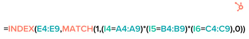
The components begins together with your GPS, which is the INDEX serve as. You’re on the lookout for the variance, so you choose rows E4 thru E9, as this is the place the solution will probably be.
3. Upload your levels.
The extra columns you may have, the extra levels you’ll want to upload to slender down your effects.
As a reminder, you’re on the lookout for the variance for an match that had a $10,000 price range and had a goal of birthday party. Which means you’ll have to inform Excel which rows hang the
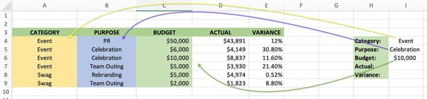
Beginning with the “match,” standards, you to find it first in I4., with its vary situated in column A between rows 4 and 9.
Practice the similar procedure for “birthday party” – it’s in I5 and its vary is B4 and B9. Finally, the “$10,000” is in I6, with a variety of C4 thru C9.
The ultimate step this is so as to add 0, because of this you’re on the lookout for a precise fit.
That’s how you find yourself with this ultimate components:
4. Run the components.
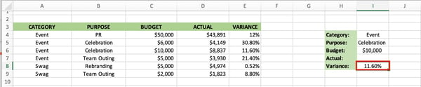
As a result of that is an array components, you should press Ctrl+Shift+Input to get the precise effects, except you might be the usage of Excel 365.
There you may have it!

![]()