Coordinating a large quantity of knowledge in Microsoft Excel is a time-consuming headache. That headache may also be made even worse when you wish to have to check knowledge throughout more than one spreadsheets. The very last thing you need to do is manually switch cells the usage of replica and paste. Fortunately, you do not need to. The VLOOKUP serve as assist you to automate this job and prevent heaps of time.
I do know, “VLOOKUP serve as” sounds just like the geekiest, most complex factor ever. However by the point you end studying this newsletter, you’ll be able to surprise the way you ever survived in Excel with out it.
Microsoft Excel’s VLOOKUP serve as is more uncomplicated to make use of than you assume. What is extra, it’s extremely robust, and is without a doubt one thing you need to have on your arsenal of analytical guns.What does VLOOKUP do, precisely? Here is the straightforward rationalization: The VLOOKUP serve as searches for a particular price on your knowledge, and as soon as it identifies that price, it will possibly to find — and show — any other piece of knowledge that is related to that price.
VLOOKUP stands for “vertical look up.” In Excel, this implies the act of having a look up knowledge vertically throughout a spreadsheet, the usage of the spreadsheet’s columns — and a novel identifier inside the ones columns — as the foundation of your seek. Whilst you glance up your knowledge, it should be indexed vertically anywhere that knowledge is positioned.
The formulation at all times searches to the correct.
When accomplishing a VLOOKUP in Excel, you are necessarily in search of new knowledge in a distinct spreadsheet this is related to previous knowledge on your present one. When VLOOKUP runs this seek, it at all times appears to be like for the brand new knowledge to the appropriate of your present knowledge.
For example, if one spreadsheet has a vertical checklist of names, and some other spreadsheet has an unorganized checklist of the ones names and their electronic mail addresses, you’ll be able to use VLOOKUP to retrieve the ones electronic mail addresses within the order you’ve got them on your first spreadsheet. The ones electronic mail addresses should be indexed within the column to the correct of the names in the second one spreadsheet, or Excel will be unable to search out them. (Pass determine … )
The formulation wishes a novel identifier to retrieve knowledge.
The name of the game to how VLOOKUP works? Distinctive identifiers.
A novel identifier is a work of knowledge that either one of your knowledge assets percentage, and — as its identify implies — it’s distinctive (i.e. the identifier is simplest related to one report on your database). Distinctive identifiers come with product codes, stock-keeping gadgets (SKUs), and buyer contacts.
Alright, sufficient rationalization: let’s examine some other instance of the VLOOKUP in motion!
VLOOKUP Instance
Within the video under, we will display an instance in motion, the usage of the VLOOKUP serve as to compare electronic mail addresses (from a 2nd knowledge supply) to their corresponding knowledge in a separate sheet.
Writer’s be aware: There are lots of other variations of Excel, so what you notice within the video above may no longer at all times fit up precisely with what you’ll be able to see on your model. That is why we inspire you to observe at the side of the written directions under.
To your reference, here is what a VLOOKUP serve as looks as if:
Within the steps under, we will assign the correct price to each and every of those elements, the usage of buyer names as our distinctive identifier to search out the MRR of each and every buyer.
1. Determine a column of cells you would love to fill with new knowledge.
Take note, you are looking to retrieve knowledge from some other sheet and deposit it into this one. With that during thoughts, label a column subsequent to the cells you need additional information on with a correct name within the best cellular, similar to “MRR,” for per month habitual earnings. This new column is the place the knowledge you are fetching will cross.
2. Make a selection ‘Serve as’ (Fx) > VLOOKUP and insert this formulation into your highlighted cellular.
To the left of the textual content bar above your spreadsheet, you’ll be able to see a small serve as icon that appears like a script: Fx. Click on at the first empty cellular underneath your column name after which click on this serve as icon. A field titled Method Builder or Insert Serve as will seem to the correct of your display (relying on which model of Excel you’ve got).
Seek for and make a selection “VLOOKUP” from the checklist of choices integrated within the Method Builder. Then, make a selection OK or Insert Serve as to start out construction your VLOOKUP. The cellular you now have highlighted on your spreadsheet will have to now seem like this: “=VLOOKUP()“
You’ll additionally input this formulation into a decision manually through getting into the daring textual content above precisely into your required cellular.
With the =VLOOKUP textual content entered into your first cellular, it is time to fill the formulation with 4 other standards. Those standards will lend a hand Excel slender down precisely the place the knowledge you need is positioned and what to search for.
3. Input the look up price for which you need to retrieve new knowledge.
The primary standards is your look up price — that is the price of your spreadsheet that has knowledge related to it, which you need Excel to search out and go back for you. To go into it, click on at the cellular that carries a worth you are looking for a fit for. In our instance, proven above, it is in cellular A2. You can get started migrating your new knowledge into D2, since this cellular represents the MRR of the client identify indexed in A2.
Be mindful your look up price may also be the rest: textual content, numbers, web site hyperlinks, you identify it. So long as the price you are looking up fits the price within the referring spreadsheet — which we will speak about that during your next step — this serve as will go back the knowledge you need.
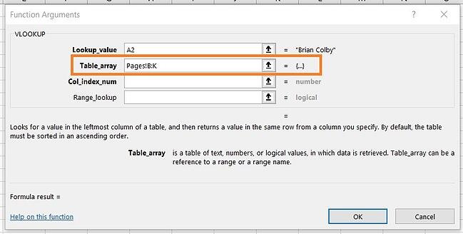
4. Input the desk array of the spreadsheet the place your required knowledge is positioned.
Subsequent to the “desk array” box, input the variability of cells you would like to go looking and the sheet the place those cells are positioned, the usage of the layout proven within the screenshot above. The access above way the knowledge we are in search of is in a spreadsheet titled “Pages” and may also be discovered any place between column B and column Ok.
The sheet the place your knowledge is positioned should be inside your present Excel record. This implies your knowledge can both be in a distinct desk of cells someplace on your present spreadsheet, or in a distinct spreadsheet related on the backside of your workbook, as proven under.
As an example, in case your knowledge is positioned in “Sheet2” between cells C7 and L18, your desk array access shall be “Sheet2!C7:L18.”
5. Input the column choice of the knowledge you need Excel to go back.
Underneath the desk array box, you’ll be able to input the “column index quantity” of the desk array you are looking via. As an example, if you are that specialize in columns B via Ok (notated “B:Ok” when entered within the “desk array” box), however the particular values you need are in column Ok, you’ll be able to input “10” within the “column index quantity” box, since column Ok is the tenth column from the left.
6. Input your vary look up to search out a precise or approximate fit of your look up price.
In eventualities like ours, which considerations per month earnings, you need to search out actual fits from the desk you are looking via. To do that, input “FALSE” within the “vary look up” box. This tells Excel you need to search out simplest the precise earnings related to each and every gross sales touch.
To respond to your burning query: Sure, you’ll be able to permit Excel to search for an approximate fit as an alternative of a precise fit. To take action, merely input TRUE as an alternative of FALSE within the fourth box proven above.
When VLOOKUP is about for an approximate fit, it is in search of knowledge that the majority carefully resembles your look up price, somewhat than knowledge that is similar to that price. If you are having a look up knowledge related to a listing of web site hyperlinks, for instance, and a few of your hyperlinks have “https://” originally, it could behoove you in finding an approximate fit simply in case there are hyperlinks that should not have this “https://” tag. This fashion, the remainder of the hyperlink can fit with out this preliminary textual content tag inflicting your VLOOKUP formulation to go back an error if Excel can not to find it.
7. Click on ‘Performed’ (or ‘Input’) and fill your new column.
As a way to formally carry within the values you need into your new column from Step 1, click on “Performed” (or “Input,” relying to your model of Excel) after filling the “vary look up” box. This will likely populate your first cellular. You could take this chance to appear within the different spreadsheet to verify this used to be the proper price.
If this is the case, populate the remainder of the brand new column with each and every next price through clicking the primary crammed cellular, then clicking the tiny sq. that looks at the bottom-right nook of this cellular. Performed! Your whole values will have to seem.
VLOOKUP No longer Running?
Should you’ve adopted the above steps and your VLOOKUP continues to be no longer operating, it’ll both be a topic together with your:
Syntax (i.e. how you’ve got structured the formulation)
Values (i.e. whether or not the knowledge it is having a look up is excellent and formatted as it should be)
Troubleshooting VLOOKUP Syntax
Get started with having a look on the VLOOKUP formulation that you’ve got written within the designated cellular.
Is it relating to the correct look up price for its key identifier?
Does it specify the proper desk array vary for the values it must retrieve
Does it specify the proper sheet for the variability?
Is that sheet spelled as it should be?
Is it the usage of the proper syntax to confer with the sheet? (e.g. Pages!B:Ok or ‘Sheet 1’!B:Ok)
Has the proper column quantity been specified? (e.g. A is 1, B is two, and so forth)
Is True or False the proper course for a way your sheet is about up?
Troubleshooting VLOOKUP Values
If the syntax isn’t the issue, how you could have a topic with the values you are looking to obtain themselves. This incessantly manifests as an #N/A error the place the VLOOKUP can not discover a referenced price.
Are the values formatted vertically and from appropriate to left?
Do the values fit the way you confer with them?
As an example, if you are having a look up URL knowledge, each and every URL should be a row with its corresponding knowledge to the left of it in the similar row. In case you have the URLs as column headers with the knowledge shifting vertically, the VLOOKUP won’t paintings.
Holding with this case, the URLs should fit in layout in each sheets. In case you have one sheet together with the “https://” within the price whilst the opposite sheet omits the “https://”, the VLOOKUP will be unable to compare the values.
VLOOKUPs as a Robust Advertising and marketing Device
Entrepreneurs have to investigate knowledge from a lot of assets to get a whole image of lead era (and extra). Microsoft Excel is the very best software to try this appropriately and at scale, particularly with the VLOOKUP serve as.
Editor’s be aware: This publish used to be at the beginning printed in March 2019 and has been up to date for comprehensiveness.
![Download 9 Excel Templates for Marketers [Free Kit]](https://wpfixall.com/wp-content/uploads/2021/07/9ff7a4fe-5293-496c-acca-566bc6e73f42.png.webp)