Create a Pivot Desk in Excel: A Step-by-Step Educational

The pivot desk is one among Microsoft Excel’s maximum robust — and intimidating — purposes. Robust as it help you summarize and make sense of huge information units. Intimidating since you’re now not precisely an Excel knowledgeable, and pivot tables have all the time had a name for being difficult.

The excellent news: Finding out create a pivot desk in Excel is way more uncomplicated than you could’ve been resulted in imagine.

However earlier than we stroll you during the procedure of constructing one, let’s take a step again and remember to perceive precisely what a pivot desk is, and why you could want to use one.

In different phrases, pivot tables extract that means from that apparently never-ending jumble of numbers to your display screen. And extra in particular, it means that you can team your information in numerous techniques so you’ll be able to draw useful conclusions extra simply.

The “pivot” a part of a pivot desk stems from the truth that you’ll be able to rotate (or pivot) the information within the desk to view it from a special point of view. To be transparent, you are now not including to, subtracting from, or differently converting your information when you are making a pivot. As a substitute, you are merely reorganizing the information so you’ll be able to disclose helpful data from it.

What are pivot tables used for?

If you are nonetheless feeling just a little puzzled about what pivot tables in truth do, do not be concerned. That is a kind of applied sciences which are a lot more uncomplicated to know as soon as you have noticed it in motion.

The aim of pivot tables is to provide user-friendly techniques to briefly summarize huge quantities of knowledge. They may be able to be used to raised perceive, show, and analyze numerical information intimately — and will lend a hand establish and resolution unanticipated questions surrounding it.

Listed below are seven hypothetical eventualities the place a pivot desk generally is a answer:

1. Evaluating gross sales totals of various merchandise.

Say you’ve gotten a worksheet that comprises per thirty days gross sales information for 3 other merchandise — product 1, product 2, and product 3 — and you wish to have to determine which of the 3 has been bringing in essentially the most greenbacks. You’ll want to, in fact, glance during the worksheet and manually upload the corresponding gross sales determine to a working general each time product 1 seems. You’ll want to then do the similar for product 2, and product 3 till you’ve gotten totals for they all. Piece of cake, appropriate?

Now, believe your per thirty days gross sales worksheet has tens of millions of rows. Manually sorting thru all of them may just take an entire life. The usage of a pivot desk, you’ll be able to mechanically combination all the gross sales figures for product 1, product 2, and product 3 — and calculate their respective sums — in not up to a minute.

2. Appearing gross sales as percentages of general gross sales.

Pivot tables naturally display the totals of each and every row or column whilst you create them. However that isn’t the one determine you’ll be able to mechanically produce.

Let’s assume you entered quarterly gross sales numbers for 3 separate merchandise into an Excel sheet and grew to become this knowledge right into a pivot desk. The desk would mechanically provide you with 3 totals on the backside of each and every column — having added up each and every product’s quarterly gross sales. However what in case you sought after to seek out the proportion those gross sales contributed to all corporate gross sales, moderately than simply the ones merchandise’ gross sales totals?

With a pivot desk, you’ll be able to configure each and every column to provide the column’s proportion of all 3 column totals, as an alternative of simply the column general. If 3 gross sales totaled $200,000 in gross sales, as an example, and the primary product made $45,000, you’ll be able to edit a pivot desk to as an alternative say this product contributed 22.5% of all corporate gross sales.

To turn gross sales as percentages of general gross sales in a pivot desk, merely right-click the cellular sporting a gross sales general and make a selection Display Values As > % of Grand General.

3. Combining reproduction information.

On this situation, you have simply finished a weblog redesign and needed to replace a number of URLs. Sadly, your weblog reporting device did not maintain it really well and ended up splitting the “view” metrics for unmarried posts between two other URLs. So to your spreadsheet, you’ve gotten two separate cases of each and every particular person weblog publish. To get correct information, you want to mix the view totals for each and every of those duplicates.

That is the place the pivot desk comes into play. As a substitute of getting to manually seek for and mix the entire metrics from the duplicates, you’ll be able to summarize your information (by means of pivot desk) via weblog publish name, and voilà: the view metrics from the ones reproduction posts will probably be aggregated mechanically.

4. Getting an worker headcount for separate departments.

Pivot tables are useful for mechanically calculating issues that you’ll be able to’t simply in finding in a fundamental Excel desk. A kind of issues is counting rows that each one have one thing in not unusual.

When you’ve got a listing of workers in an Excel sheet, for example, and subsequent to the workers’ names are the respective departments they belong to, you’ll be able to create a pivot desk from this knowledge that presentations you each and every division title and the choice of workers that belong to these departments. The pivot desk successfully removes your job of sorting the Excel sheet via division title and counting each and every row manually.

5. Including default values to drain cells.

Now not each dataset you input into Excel will populate each cellular. If you are looking forward to new information to come back in earlier than coming into it into Excel, you may have a whole lot of empty cells that glance complicated or want additional clarification when appearing this knowledge for your supervisor. That is the place pivot tables are available in.

You’ll be able to simply customise a pivot desk to fill empty cells with a default worth, equivalent to $0, or TBD (for “to be decided”). For massive tables of knowledge, having the ability to tag those cells briefly is an invaluable characteristic when many of us are reviewing the similar sheet.

To mechanically layout the empty cells of your pivot desk, right-click your desk and click on PivotTable Choices. Within the window that looks, take a look at the field categorised Empty Cells As and input what you need displayed when a cellular has no different worth.

Create a Pivot Desk

Input your information into a spread of rows and columns.
Kind your information via a particular characteristic.
Spotlight your cells to create your pivot desk.
Drag and drop a box into the “Row Labels” house.
Drag and drop a box into the “Values” house.
Fantastic-tune your calculations.

Now that you’ve got a greater sense of what pivot tables can be utilized for, let’s get into the nitty-gritty of in truth create one.

Step 1. Input your information into a spread of rows and columns.

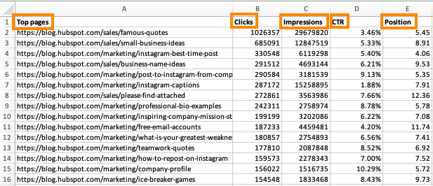
Each and every pivot desk in Excel begins with a fundamental Excel desk, the place your entire information is housed. To create this desk, merely input your values into a particular set of rows and columns. Use the topmost row or the topmost column to categorize your values via what they constitute.

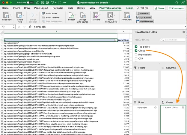
As an example, to create an Excel desk of weblog publish efficiency information, you may have a column record each and every “Best Pages,” a column record each and every URL’s “Clicks,” a column record each and every publish’s “Impressions,” and so forth. (We’re going to be the use of that instance within the steps that practice.)

Step 2. Kind your information via a particular characteristic.

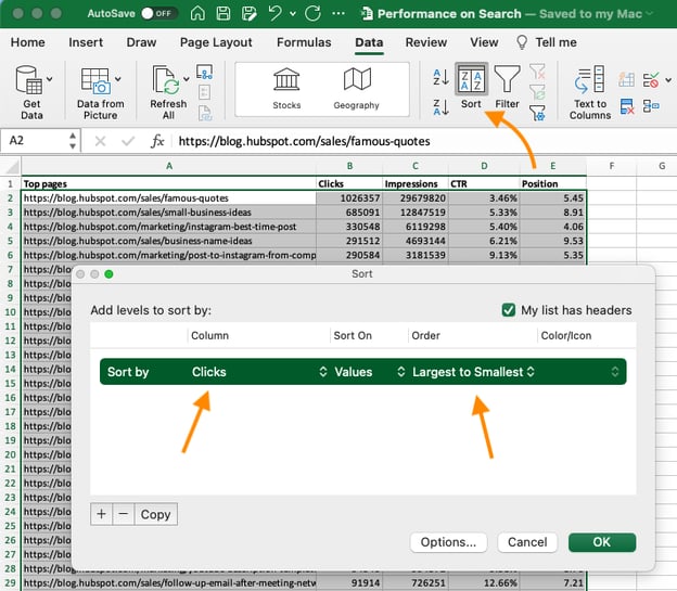
If in case you have the entire information you wish to have entered into your Excel sheet, you will want to type this knowledge by hook or by crook so it is more uncomplicated to control if you flip it right into a pivot desk.

To type your information, click on the Knowledge tab within the best navigation bar and make a selection the Kind icon beneath it. Within the window that looks, you’ll be able to decide to type your information via any column you wish to have and in any order.

As an example, to type your Excel sheet via “Perspectives to Date,” make a selection this column name below Column after which make a selection whether or not you wish to have to reserve your posts from smallest to biggest, or from biggest to smallest.

Make a choice OK at the bottom-right of the Kind window, and you’ll be able to effectively reorder each and every row of your Excel sheet via the choice of perspectives each and every weblog publish has won.

Step 3. Spotlight your cells to create your pivot desk.

As soon as you have entered information into your Excel worksheet, and taken care of it for your liking, spotlight the cells you’ll love to summarize in a pivot desk. Click on Insert alongside the highest navigation, and make a selection the PivotTable icon. You’ll be able to additionally click on any place to your worksheet, make a selection “PivotTable,” and manually input the variability of cells you need integrated within the PivotTable.

This may occasionally open an choice field the place, along with atmosphere your cellular vary, you’ll be able to make a selection whether or not or to not release this pivot desk in a brand new worksheet or stay it within the current worksheet. Should you open a brand new sheet, you’ll be able to navigate to and clear of it on the backside of your Excel workbook. As soon as you have selected, click on OK.

On the other hand, you’ll be able to spotlight your cells, make a selection Really useful PivotTables to the appropriate of the PivotTable icon, and open a pivot desk with pre-set ideas for prepare each and every row and column.

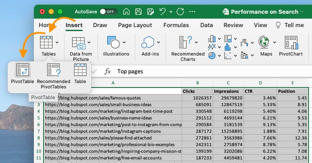
Notice: If you are the use of an previous model of Excel, “PivotTables” could also be below Tables or Knowledge alongside the highest navigation, moderately than “Insert.” In Google Sheets, you’ll be able to create pivot tables from the Knowledge dropdown alongside the highest navigation.

Step 4. Drag and drop a box into the “Row Labels” house.

After you have finished Step 3, Excel will create a clean pivot desk for you. The next move is to pull and drop a box — categorised in keeping with the names of the columns to your spreadsheet — into the Row Labels house. This may occasionally resolve what distinctive identifier — weblog publish name, product title, and so forth — the pivot desk will prepare your information via.

As an example, shall we say you wish to have to prepare a number of running a blog information via publish name. To do this, you’ll merely click on and drag the “Best pages” box to the “Row Labels” house.

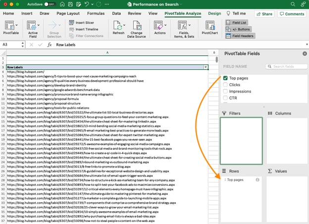
Notice: Your pivot desk would possibly glance other relying on which model of Excel you are running with. On the other hand, the overall rules stay the similar.

Step 5. Drag and drop a box into the “Values” house.

As soon as you have established what you are going to prepare your information via, the next step is so as to add in some values via dragging a box into the Values house.

Sticking with the running a blog information instance, shall we say you wish to have to summarize weblog publish perspectives via name. To try this, you’ll merely drag the “Perspectives” box into the Values house.

Step 6. Fantastic-tune your calculations.

The sum of a selected worth will probably be calculated via default, however you’ll be able to simply exchange this to one thing like reasonable, most, or minimal relying on what you wish to have to calculate.

On a Mac, you’ll be able to do that via clicking at the small i subsequent to a price within the “Values” house, settling on the choice you wish to have, and clicking “OK.” If you’ve made your variety, your pivot desk will probably be up to date accordingly.

If you are the use of a PC, you’ll be able to want to click on at the small upside-down triangle subsequent for your worth and make a selection Price Box Settings to get entry to the menu.

Whilst you’ve labeled your information for your liking, save your paintings and use it as you please.

Digging Deeper With Pivot Tables

You could have now discovered the fundamentals of pivot desk advent in Excel. With this working out, you’ll be able to work out what you want out of your pivot desk and in finding the answers you’re in search of.

As an example, chances are you’ll understand that the information to your pivot desk is not taken care of the way in which you need. If that is so, Excel’s Kind serve as help you out. On the other hand, chances are you’ll want to incorporate information from any other supply into your reporting, wherein case the VLOOKUP serve as may just turn out to be useful.

Editor’s notice: This publish was once at first printed in December 2018 and has been up to date for comprehensiveness.