Let’s fake you could have a spreadsheet with 1,000 rows of information — it might be beautiful tricky to identify patterns within the information with the bare eye. Input conditional formatting.
![Download 10 Excel Templates for Marketers [Free Kit]](https://wpfixall.com/wp-content/uploads/2021/07/9ff7a4fe-5293-496c-acca-566bc6e73f42.png.webp)
This robust device highlights cells that meet a selected situation or “rule.” In different phrases, it brings your spreadsheet to existence by means of including colour to patterns and tendencies.
Right here, we’re going to quilt tips on how to observe, edit, and replica and paste conditional formatting.
Contents
Conditional Formatting In response to Textual content
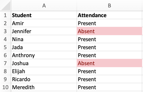
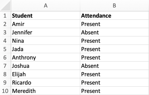
On this instance, let’s use conditional formatting to an attendance record to focus on who was once absent. The picture beneath is the information set I’ll use to run via this rationalization:
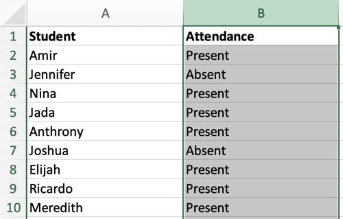
1. First, make a selection the column or row you wish to have to use conditional formatting to. On this case, we’re going to make a selection column B.
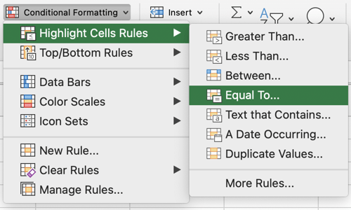
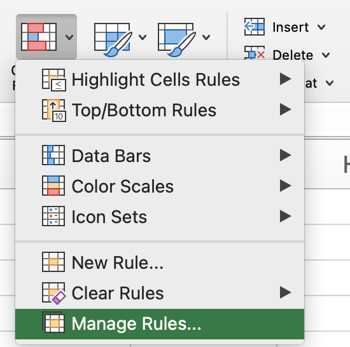
2. To spotlight who was once absent, navigate to the header toolbar and make a selection Conditional Formatting, as proven within the symbol beneath.

3. When the Conditional Formatting drop-down menu seems, make a selection Spotlight Cells Regulations, then Equivalent To.
4. Within the New Formatting conversation field, alternate Mobile Worth to Particular Textual content. Then, sort “Absent” within the textual content field. Reference the picture beneath:
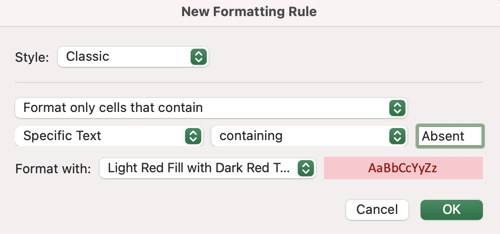
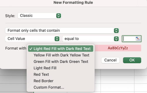
5. From the New Formatting conversation field, we will additionally select how we wish to structure the cells containing the phrase “Absent.” Take a look at the choices beneath.
For this situation, let’s stick to the default possibility (Gentle Crimson Fill with Darkish Crimson Textual content).
6. Click on OK. Now — due to conditional formatting — we will briefly establish which scholars have been absent.
Within the subsequent phase, we’re going to quilt tips on how to observe conditional formatting in accordance with some other cellular within the spreadsheet.
Conditional Formatting In response to Some other Mobile
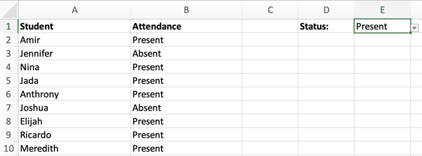
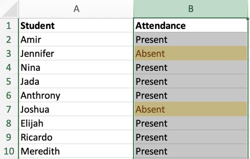
On this instance, the objective is to focus on the cells that fit the drop-down menu in cellular E1. The picture beneath is the pattern information set I’ll use for this rationalization:
1. First, make a selection column B.
2. Navigate to the header toolbar and make a selection Conditional Formatting. When the Conditional Formatting drop-down menu seems, make a selection Spotlight Cells Regulations, then Equivalent To.
3. Within the New Formatting conversation field, make a selection Mobile Worth and Equivalent To.
Within the textual content field, you’ll be able to both click on your mouse on cellular E1 (the cellular that accommodates the drop-down menu), or manually input the method =$E$1. See beneath.
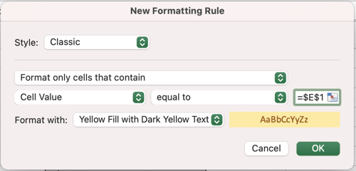
4. As you’ll be able to see within the symbol above, we additionally modified the formatting to Yellow Fill with Darkish Yellow Textual content. On the other hand, you’ll be able to alternate this selection in your desire. Click on OK.
5. Now, the cells that fit cellular E1 are highlighted in yellow. Realize how the highlighted cells alternate relying at the standing:
- When the standing is Provide:

- When the standing is Absent:
Methods to Edit Conditional Formatting
Here is some excellent information — conditional formatting is now not set in stone, that means you’ll be able to edit or delete it later. Listed below are the stairs to try this:
1. Get started by means of deciding on the cellular (or cellular vary) that accommodates a conditional formatting rule.
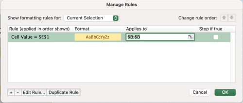
2. Navigate to the header toolbar and make a selection Conditional Formatting, then Set up Regulations.
3. The Set up Regulations conversation field will record the present laws to your variety. Make a choice the guideline you wish to have to edit and click on Edit Rule.
Methods to Reproduction Conditional Formatting in Excel
You’ll be able to simply reproduction a conditional formatting rule to some other cellular to (or vary of cells) by means of the use of one of the most following approaches.
1. Easy reproduction/paste.
The primary manner is somewhat simple. Get started by means of deciding on the cellular you wish to have to duplicate and hit the Reproduction button within the header toolbar — or click on Keep an eye on-C (or Command-C on a Mac).
Then, make a selection the objective cellular and hit the Paste button within the header toolbar, or click on Keep an eye on-V (or Command-V on a Mac).
2. Structure Painter
The second one manner makes use of the device Structure Painter, which is positioned within the header toolbar. Take a look at the picture beneath:

To begin, click on at the cellular you wish to have to duplicate, then click on Structure Painter. Your mouse icon will alternate to a paintbrush. Then, drag the paintbrush to the cellular (or vary of cells) the place you wish to have to stick the structure. Finally, to forestall the use of the paintbrush, press Esc for your keyboard.
Conditional formatting is an impressive strategy to visualize the information on your spreadsheet. With only a few clicks, you’ll be able to emphasize essential tendencies or patterns you will have in a different way neglected. With the guidelines on this put up, you’ll be capable of use Conditional Formatting to its fullest extent.

![]()