Reproduction knowledge is the bane of spreadsheet answers, particularly at scale. Given the amount and number of knowledge now entered by way of groups, it’s conceivable that copy knowledge in equipment like Google Sheets is also related and vital, or it generally is a irritating distraction from the main function of spreadsheet efforts.
The prospective downside raises a excellent query: How do you spotlight duplicates in Google Sheets?
We’ve were given you lined with a step by step have a look at find out how to spotlight duplicates in Google Sheets, entire with pictures to be sure to’re not off course in terms of de-duplicating your knowledge.
![→ Access Now: Google Sheets Templates [Free Kit]](https://wpfixall.com/wp-content/uploads/2022/01/e7cd3f82-cab9-4017-b019-ee3fc550e0b5.png.webp)
Contents
- 1 Highlighting Reproduction Knowledge in Google Sheets
- 2 Step-by-Step: Learn how to Spotlight Duplicates in Google Sheets (With Photos)
- 2.1 Step 1: Open your spreadsheet.
- 2.2
- 2.3 Step 2: Spotlight the information you wish to have to test.
- 2.4 Step 3: Below “Layout”, choose “Conditional Formatting.”
- 2.5 Step 4: Make a choice “Customized system is.”
- 2.6 Step 5: Input the customized replica checking system.
- 2.7 Step 6: Click on “Completed” to look the effects.
- 3 Learn how to Spotlight Duplicates in More than one Rows and Columns
- 4 Dealing With Duplicates in Duplicates in Google Sheets
Highlighting Reproduction Knowledge in Google Sheets
Google Sheets is a unfastened, cloud-based selection to proprietary spreadsheet methods and — no wonder, because it’s Google we’re coping with — provides a number of serious options to assist streamline knowledge access, formatting, and calculations.

Google Sheets has the entire acquainted purposes: Document, Edit, View, Layout, Knowledge, Gear, and so on. and makes it simple to briefly input your knowledge, upload formulation for calculations, and uncover key relationships. What Sheets doesn’t have, alternatively, is a simple technique to in finding and spotlight duplicates.
Whilst different spreadsheet equipment, akin to Excel, have integrated conditional formatting equipment that may pinpoint replica knowledge for your sheet, Google’s resolution calls for somewhat extra guide effort.
Step-by-Step: Learn how to Spotlight Duplicates in Google Sheets (With Photos)
So how do you mechanically spotlight duplicates in Google Sheets? Whilst there’s no integrated software for this function, you’ll leverage some integrated purposes to focus on replica knowledge.
Right here’s a step by step information:
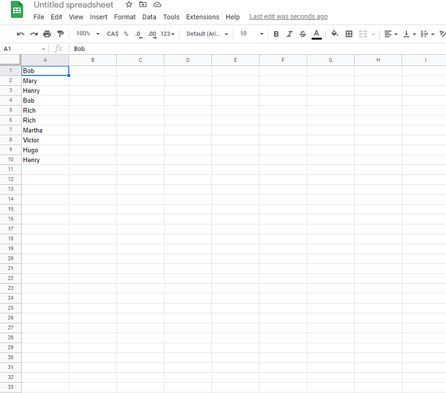
Step 1: Open your spreadsheet.
Step 2: Spotlight the information you wish to have to test.
Step 3: Below “Layout”, choose “Conditional Formatting.”
Step 4: Make a choice “Customized system is.”
Step 5: Input the customized replica checking system.
Step 6: Click on “Completed” to look the effects.
Step 1: Open your spreadsheet.
First, head to Google Sheets and open the spreadsheet you wish to have to test for replica knowledge.

Step 2: Spotlight the information you wish to have to test.
Subsequent, left-click and drag your cursor over the information you wish to have to test to focus on it.

Step 3: Below “Layout”, choose “Conditional Formatting.”
Now, head to “Layout” within the best menu row and choose “Conditional Formatting”. You will get a notification that claims “mobile isn’t empty” — if this is the case, click on on it, and also you must see this:

Step 4: Make a choice “Customized system is.”
Subsequent, we wish to create a customized system. Below “Layout cells if”, choose the drop-down menu and scroll all the way down to “Customized system is”.

Step 5: Input the customized replica checking system.
To seek for replica knowledge, we wish to input the customized replica checking system, which for our column of knowledge looks as if this:
=COUNTIF(A:A,A1)>1
This system searches for any textual content string that looks greater than as soon as in our decided on knowledge set, and by way of default will spotlight it in inexperienced. For those who favor a distinct colour, click on at the small paint pot icon within the formatting taste bar and choose the colour you favor.

Step 6: Click on “Completed” to look the effects.
And voilà — we’ve highlighted the replica knowledge in Google Sheets.

Learn how to Spotlight Duplicates in More than one Rows and Columns
For those who’ve were given a bigger knowledge set to test, it’s additionally conceivable to focus on knowledge duplicates in a couple of columns or rows.
This begins the similar manner because the replica checking procedure above — the one distinction is that you simply trade the information vary to incorporate the entire cells you wish to have to match.
In apply, this implies getting into an expanded knowledge vary within the Conditional structure regulations menu and the customized structure field. Let’s use the instance above as a kick off point, however as an alternative of simply looking out column A for duplicates, we’re going to go looking throughout 3 columns: A, B, and C, and in addition throughout rows 1-10.

After we input our conditional structure regulations, Practice to Vary turns into A1:C10 and our customized system turns into:
=COUNTIF($A$2:G,Oblique(Cope with(Row(),Column(),)))>1
This may spotlight all duplicates throughout all 3 columns and all 10 rows, making it simple to identify knowledge doppelgangers:

Dealing With Duplicates in Duplicates in Google Sheets
Are you able to spotlight duplicates in Google Sheets? Completely. Whilst the method takes extra effort than any other spreadsheet answers, it’s simple to duplicate whenever you’ve completed it a few times, and whenever you’re happy with the method you’ll scale as much as in finding duplicates throughout rows, columns, or even a lot higher knowledge units.

![]()